
Introduction to PID Feed Forward
PID Feed Forward allows you to immediately compensate for a change before Proportional, and Integral have a chance to act. It does this by BIASing the control variable. For example, consider a tank where we need to maintain a constant level. As soon as we start removing more product from the tank, we can immediately increase the control variable. This will immediately raise the supply of product back into the tank. In this case, we’re setting this up on a simulator. If this is a real process, be sure to take all necessary precautions. This is for example only. The setup will be different on your own processes.
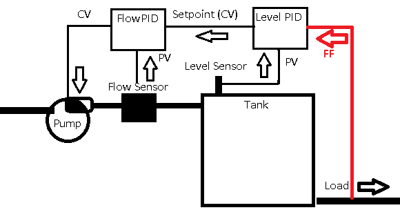
Likewise, if we reduce the load, we can immediately reduce the control variable to slow down flow into the tank.
In the last section, we configured a cascading PIDE Loop. We’ll build on that work in this section.
Without PID Feed Forward
Without PID Feed Forward, even though our load has increased, the Flow Controller does not know if this is due to a simple fluctuation, or if the load is different. For this reason, the Feed Forward acts directly on the control variable to anticipate a drop or rise in tank level.
Let’s look at our graph without Feed Forward. As you can see, when the load reduces, the flow into the tank does not immediately change. This caused a rise in tank level. In fact, we are in danger of overfilling the tank. Likewise, when the load increases, the PID controller has to see the error before it reacts. The reaction time is very slow.
We know that derivative can help with this somewhat. However, the tank level still has to change before the PID controller reacts in any way.
Getting the PID Feed Forward Value
In this case, the Feed Forward value will be on an analog input module. This represents the current load on the system. Other processes could simply be the speed of a drive, or a valve command or position. Before we begin, let’s create a tag to point to our analog input module. We’re using channel 1 of the 1794-IE8 module.
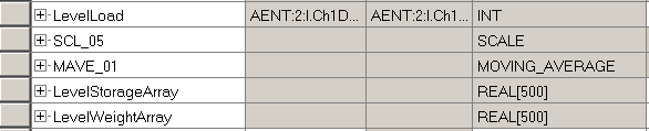
You do not need to create the tags for the SCL and MAVE instructions. Studio 5000 automatically creates them for you. This happens when you add the logic to a function block routine.
The LevelLoad tag is an alias to Channel 1 of the flex analog module. Our LevelLoad is very noisy, so we’ll want to filter this. There are many ways to filter an analog signal. For now, just create LevelStorageArray, and LevelWeightArray. They are both REAL[500]. Later on, we can reduce this array size once we find out the best filtering technique.
Add the Function Block Logic
At this point, you are ready to set up the function blocks. We’ll need an IREF, and SCL, and a MAVE (Moving Average) instruction.
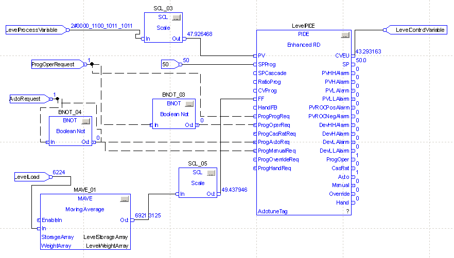
Set up your logic as follows:
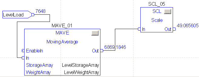
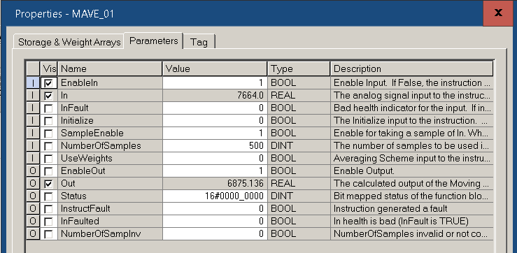
Your MAVE Configuration is very simple. Simply point the StorageArray, and the WeightArray to the two tags we just created.
Here is the configuration for the MAVE. For now, we will let it work through 500 elements to get an average, one per scan. Remember, we can work with this later to minimize the array size to reduce the memory we consume.
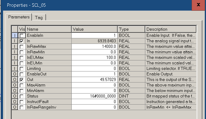
Likewise, here is our setup for the SCL Instruction. If you are unsure of raw low and raw high, simply increase the load to 100%, then back down to 0 to get your range. We will scale our signal to 100%. It’s important to realize that in this case, when the load increases, we want the control variable to increase. In some cases, you might want to scale the opposite direction. Be sure to scale in the right direction for your process! Additionally, you may not want a 1 to 1 scale. Remember, the velocity loop cares more about changes than position. If we only wanted half the Feed Forward effect, we would simply scale 0 to 50% instead of 0 to 100%.
Finally, the output of your scale connects to the FF input of the PIDE Instruction.
Realize that adding Feed Forward WILL disrupt your process. That is unless you set it up in such a way that the LevelLoad tag is “tared” at zero. Finalize your edits. Add LevelPIDE.FF to your trend chart while we wait for the loop to settle.
Test Your Work!
At last, we are ready to see the effect of our changes. We’ll compare this to the snapshot of our chart without Feed Forward.
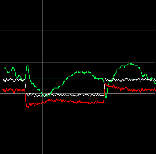
Let’s try our load transition to 40%, and let the Process Variable Settle. After that, we’ll change our load back to 50%. Again, we’ll let the Process Variable settle, and compare the results.
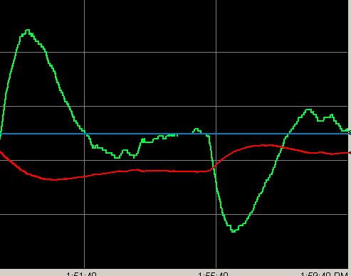
On this chart, I’m representing the Setpoint as blue. Additionally, I’m showing the Feed Forward as White. Red is our control variable, while green is our process variable.
Compare this graph to the graph without Feed Forward. Clearly, you can see that Feed Forward is helping to stay closer to the setpoint. Additionally, we don’t have as much risk of overfilling or emptying the tank.
Lead and Lag
Sometimes, you don’t want the FF input to change quickly. In this case, you might run your value through a LeadLag (LDLG) instruction before sending the value into the PID. Visit this post for the LDLG instruction. This is available in both function block and structured text languages.
Summary
In short, feed forward will bias the control variable. This allows the loop to take immediate action when we have a large change in load. Be careful to scale your feed forward properly. Ensure that it changes the control variable in the right direction. You can change the amount of feed forward action through your SCL instruction.
— Ricky Bryce