
Introduction to PlantPAx 4 PID
We typically use the PlantPAx 4 PID (P_PIDE) in closed loop controls. For example, we have a heating process. This heating process provides a control value (CV) to the heat bands. We monitor the process variable (PV) to see what effect our output has. Our goal is to maintain a desired setpoint (SP). For the same reason, we might control a tank level, or a flow rate in other closed loop systems. In a closed loop system, we provide an output, and observe (through feedback) what effect the output has.
It’s important to realize that Function Block PIDEs work differently than Ladder Logic PIDs. Function block PIDEs are velocity based, whereas ladder logic PIDs are based on traditional position algorithm. In other words, your changes will cause less of a “Bump” in the system. In other words, if the PV remains at 0, and the setpoint is 10 with a Kp of 1 (and no Integral or Derivative), your output will be 10%. However, if you change Kp to 2, and increase the SP to 20, your output would go to 30 instead of 20 like you might expect from the positional PIDs.
Remember, this document is an example only, and your actual application may vary widely.
Set up the PlantPAx 4 PID
At this time, I’ll assume that you have already started a new FactoryTalk View SE Project. I’ll also assume that you have setup the required components for a basic PlantPAx project using the 4.1 process library. If you have not done so, you will also need to import the P_PIDE add on instruction, and the required GFX files into your FactoryTalk View SE project. You will find this starting at page 75 of Rockwell’s guide.
PID Logic
In this case, I’ve created a task in Studio 5000 that executes every 1000ms. Also, I’ve created a Function block subroutine, and used the JSR statement to jump to this subroutine from the MainRoutine.
Within the Function Block, our P_PIDE is set up as follows:
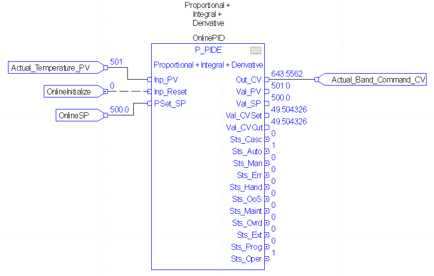
In this case, we are simulating a heating process. We are observing the actual temperature, and determining the output levels we need to provide to achieve and hold this temperature as close as possible. Even under load disturbances, the Actual_Temperature_PV should come back to the setpoint of 500. Although this is just a simulation, the Actual_Temperature_PV could alias a real world analog channel to get the temperature. The Actual_Band_Command_CV might alias an analog output channel. Be sure your process variable is updating 5 to 10 times faster than the loop execution time. (Go to the properties of the module and verify the RTS (real time sampling).
We’ll download the work, go online, and take the processor to Run or Remote Run mode.
FactoryTalk View Display
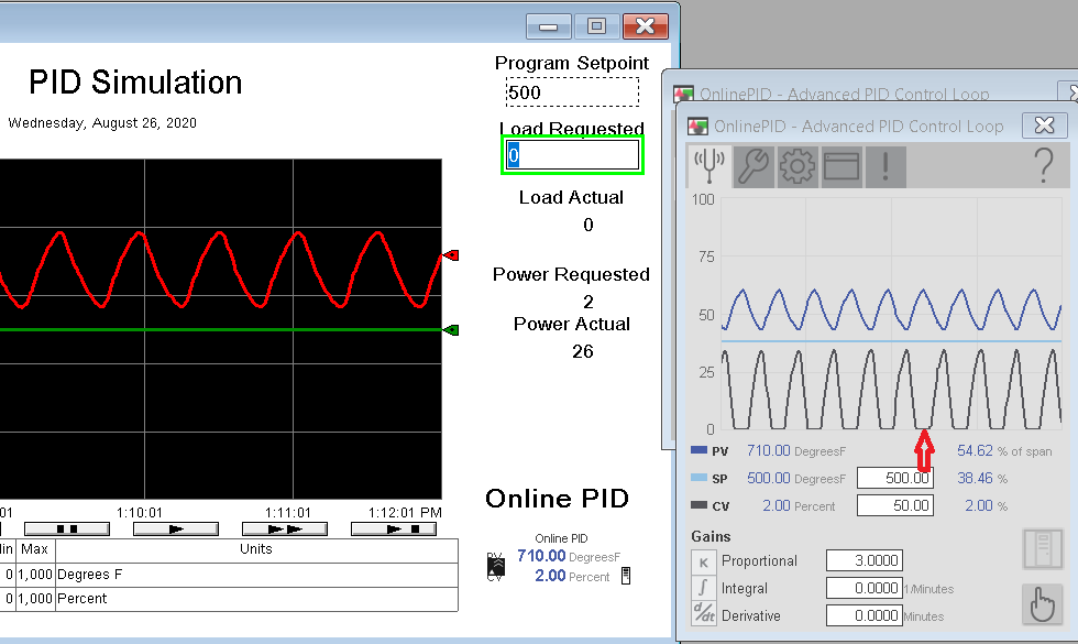
We have a display screen in FactoryTalk view that appears as follows:
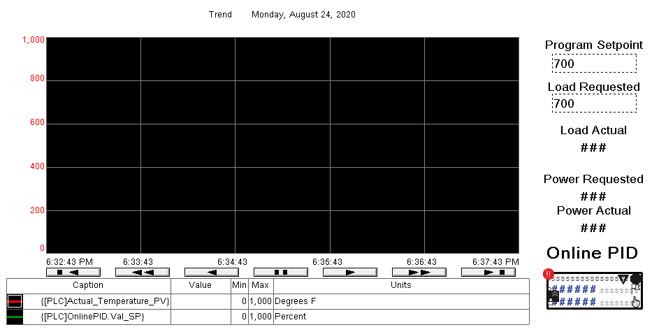
In this case, we have a trend chart that is monitoring the Actual_Temperature_PV, and the PID’s setpoint. On the right of the chart, we can adjust the setpoint, and the system load. Above all, I’ve added the very first global object out of the P_PID Graphics library. I’ve set the global object parameters on this object to point to the P_PIDE instruction’s tag.
Launch the SE Client.
Configure the P_PIDE using PlantPAx.
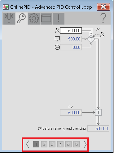
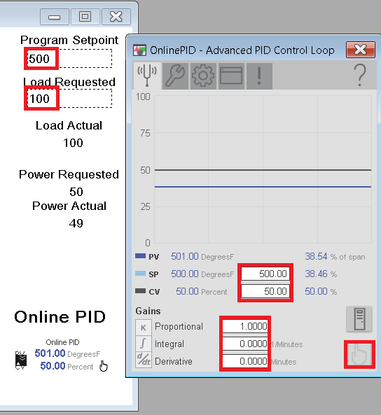
Now that the client is running, we are ready to configure the object. Click the P_PIDE object in the bottom right corner of the graphics display. Verify that you are in operator mode for this lesson.
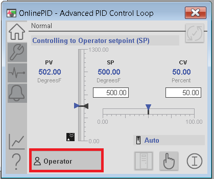
Go to Maintenance, Display Advanced Properties, and we will end up on the Tune tab. Remember, this is just for training, and to understand the effects of changes in variables. You will have to understand the risks, and take precautions when tuning a live system. To begin, set our Proportional gain to 1, and the Setpoint to 500. Integral and Derivative will start at 0. I’ve already determined that 50% power is required to achieve the SP under full (100%) load, so we will start with this setting.
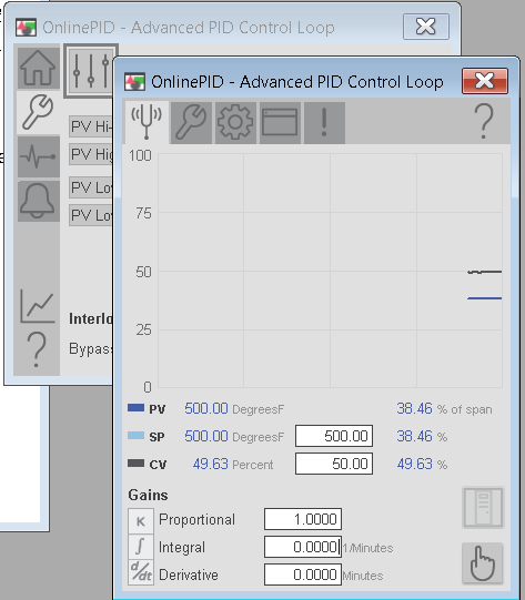
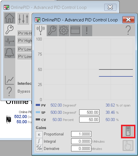
While we are here, observe the maintenance tab. Take a look at the different displays you have access to for troubleshooting.
On the Engineering tab, be sure your execution time matches actual.
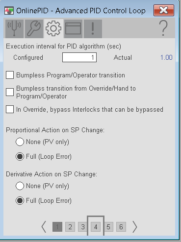
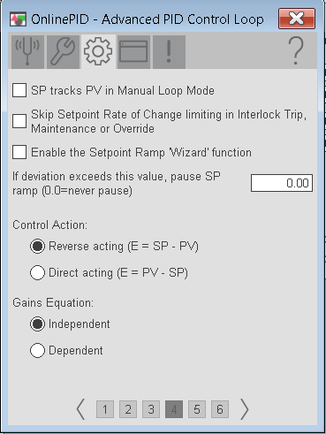
Another important setting is the Control Action, and the Algorithm. In this case, more power should decrease the error, so this loop is reverse acting. Also, I’m going to use the default (Independent) algorithm.
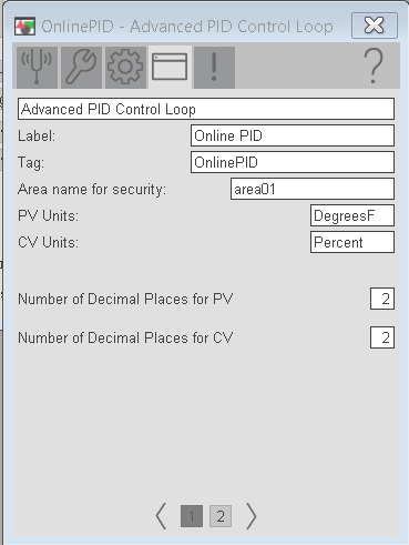
Verify the HMI Configuration is set up as follows:
Be sure your settings are as follows, and go to “Manual”. Realize that in manual mode, the and output from the PID will become exactly what you have entered on the face plate. In other words your manual CV entry will be sent directly to the output of the PID.
Notice that you are close to the setpoint.
Tuning the PlantPAx 4 PID
Now that we have everything configured, let’s get a feel for how the loop responds by doing some manual tuning.
Proportional: In a velocity based controller, this is based on the change in error.
Integral: This is based on error and time.
Derivative: Derivative is based on rate of change of error.
Our first goal is to find the “Ultimate Controller Gain”, or Ku Variable. We will start with a value of 1, and cause a disturbance. If the loop is stable, we will increase Kp to the value of 2, then to 3. Once the loop becomes unstable, we will write down the natural period in minutes. We will use this natural period for other tuning parameters. Since only Kp, and Ki are used in most applications, we will find these values. To simplify the loop, we seldom use derivative. A general rule of thumb is to then cut the Kp value in half for our starting point. Realize this method is not practical in every situation. You can research tuning methods to see which method might be best for your situation.
Find Kp
Starting with Kp=1
Let’s look at what happens when Kp=1. If you are completely unfamiliar with a process, you might start at Kp=0.1, and double each time until the loop becomes unstable. For now, take the controller to “Automatic” mode under 100% load with an SP of 500.
Start with the faceplate Maintenance | Advanced Display Properties | Engineering.
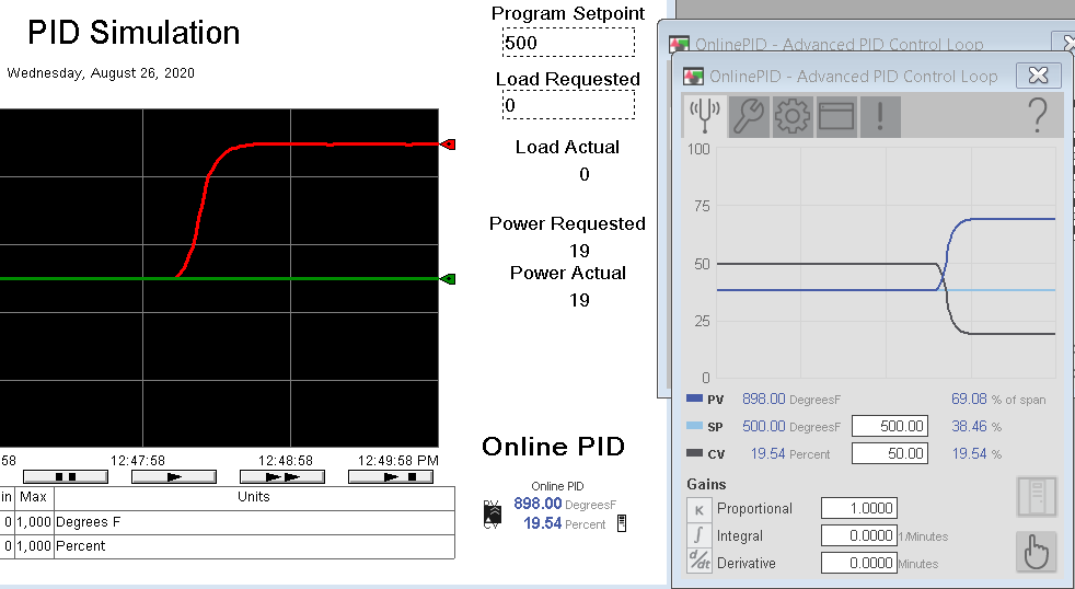
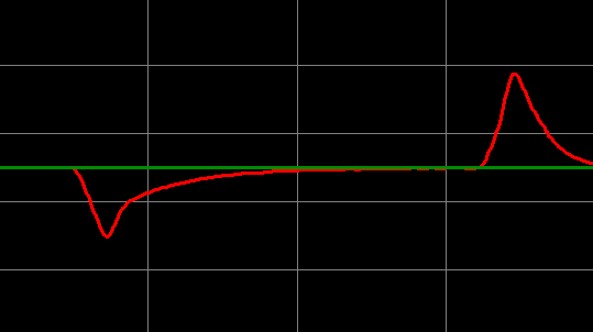
Now, set the load to 0% to cause a disturbance, and observe the action of the Process Variable. Also, notice the CV (output) drops as the PV increases.
Notice Kp=1 stabilizes.
Now, go back to Manual Mode at 100% load. Notice your power level (CV) immediately goes to 50%. Allow the loop time to stabilize.
Try Kp=2
Now, change the Kp value to 2. Put the controller back into automatic mode, and with 0% load, observe the trend charts again.
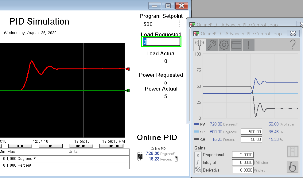
Albeit a bit more unstable, you see that our values stabilized. Again, go back to Manual Mode and set your load to 100%. Wait for the loop to stabilize.
Try Kp=3
Next, we will change the value of Kp to 3. Again, put the controller back into automatic mode with 0% load. Observe what happens. As can be seen, we are clearly unstable. Our CV is also unable to go below 0, and therefore we start to loose control.
For now, go to manual at 0% load, and set Kp to half. This value will be 1.5 as per thumb rule. Make note of the natural period (peak to peak). This appears to be around .5 minutes, and we’ll call this the Ti variable for later use.
Calculate and test Integral
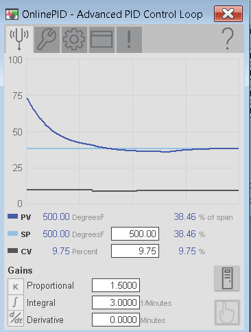
Another rule of thumb is that our Ki (since it’s in repeats per minute in this case) would be Kp/Ti, whereas Ti is the natural period. Our natural period is .5, so 1.5/.5 would give us 3. With Kp at 1.5, set Ki (Integral) to 3. Through trial and error, I’ve already determined that our setpoint needs to be to achieve the SP under no (0%) load. We need some amount of power to compensate for the ambient losses.
Allow the loop to stabilize with our new settings.
At this point, you are ready to go to Automatic mode. We’ll try various load changes. For each load change, we should always be able to get back to 500 degrees.
We could increase integral to get the loop to respond faster, but realize if we set integral too high, we could cause instability in the loop again.
Here is our integral at 3.
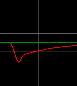
Here is our integral at 6.
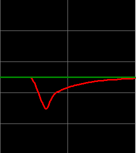
We clearly see a better response with the Integral at 6. Let’s test this when the load goes to 0.
You can see that we get back to the SP fairly quickly. We’ll leave our settings on 6 for integral. However…. Realize that we changed the slope when we made integral more aggressive. If you use Derivative, understand that derivative is based on slope, so we could indirectly have made the derivative too aggressive. Let’s try derivative to see what happens.
Calculate and test Derivative in PlantPAx 4 PID.
As I have said, derivative is seldom used, because it complicates the PID. It causes actions that are hard to determine when the process variable is noisy, such as in a flow control system. The rule of thumb for derive is that Kd=Kp(Td), where Td is 1/8 of the natural period. Therefore, Td would be .0625. (From .5/8). Kd would be 1.5 * .0625, which is .094. Let’s plug these numbers into our faceplate and observe what happens under no load and full load.
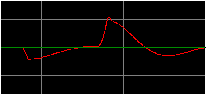
Our derivative action opposes a change in the process variable. That might be good for some applications, but we probably would not use it on this one.
Look at the effect that Derivative had on the Control Variable. I’m starting off at full load, and then I’ll go to 0 load when the PV reaches the SP. In this case, the derivative is clearly slowing down our reaction time.
For more information, visit the PlantPAx category page!
— Ricky Bryce