
Introduction to Setting up the PIDE Instruction
In this section, we’ll be Setting up the PIDE Instruction for use with our simulator. We’ll simulate a flow control process. To begin with, we’ll leave the simulator settings at default. Be sure to wire the CV from the simulator to an analog output module. Additionally, connect the PV to an analog input channel.
Set up your Tags
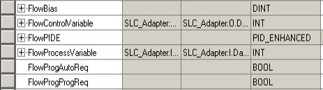
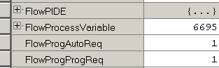
Before we begin, we need to configure some tags. We’ll need these for the PIDE instruction. , FlowProgAutoReq, and FlowProgProgReq both are BOOL. We’ll also need a FlowBias tag that is a DINT. We’ll use these later on. Create another tag called “FlowControlVariable”. This is an alias to your analog output channel. Similarly, create a tag called “FlowProcessVariable”. Be sure this is aliased to your analog input channel. Additionally, we need a workspace for the PIDE instruction. Create “FlowPIDE”, which is a PIDE_Enhanced data type.
At this point, go to “Monitor Tags”. Set the value for FlowProgAutoReq, and FlowProgProgReq both to 0.
Set up your Logic Structure
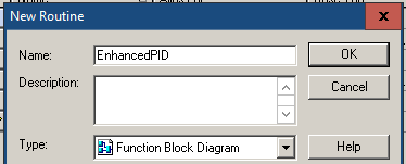
Usually, it’s best to place PID’s into a periodic task. This guarantees the update time. At this time, we’ll create a routine named “EnhancedPID”. This will be a function block type.
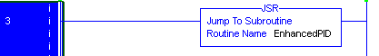
Remember to add a JSR instruction in the MainRoutine.
Add your Logic for setting up the PIDE Instruction
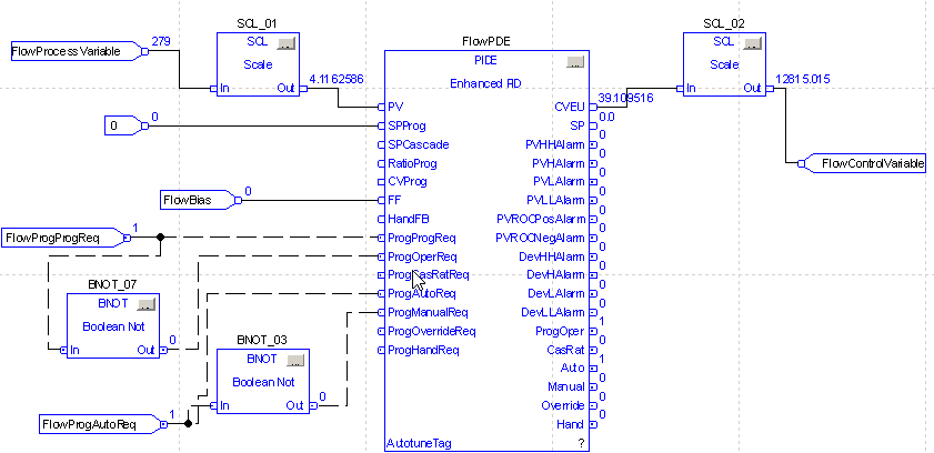
Finally, we are ready to add your logic. To start with, we’ll add the PIDE instruction. Next, we’ll add Four IREF instructions and an OREF. We also need to BNOT (Boolean NOT) instructions, and two SCL (Scale) instructions. Although we could scale the PV and CV inside of our PIDE instruction, we’ll scale this externally. This will simplify the configuration of the PIDE later on.
The first IREF instruction contains the FlowProcessVariable. Feed this through the first SCL, and into the PV node on the PIDE instruction. For the Setpoint (SP), just tie a zero into the SPProg Node. After that, we’ll need our FlowProgProgReq tag. This allows us to switch between program and operator mode via a program request. Whenever this tag has the value of 1, we will initiate a request for Program Control Mode. On the other hand, if this tag is a 0, we feed this through the BNOT to issue a program request for Operator mode.
In the same manner, we’ll set up the FlowProgAutoReq bit. Whenever this tag is high, we’ll issue an auto request. Otherwise, we’ll issue a request for manual mode (through the second BNOT instruction).
The CVEU (Control Value Engineering Units) will connect through the second SCL to the FlowControlVariable tag.
Scale Your PV and CV
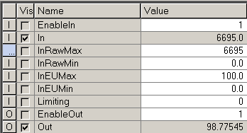
To simply the configuration of the PIDE instruction, we’ll just scale our data outside of the instruction. For the FlowProcessVariable, we need to find what the raw value is at zero %, and 100%. Monitor the FlowProcessVariable, and press the test button on your simulator. You should see a value that is near zero. Press TEST again, and you should see a raw value representing 100%. Remember these values. Don’t forget that we have a capacitor on the PV. We’ll need to let this settle out for a minute or so, then record the value. As you can see, my value is 6695. Another way to get this value is to check the user manual for the module. The simulator should send about 5v to the input channel at 100%. If you have a more advanced module, you can also check the configuration in the I/O tree.
Next, we’ll click the ellipsis on the SCL’s instruction face. This allows us to configure the instruction. A raw range of 0 to 6695 will represent 0 to 100%.
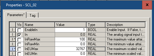
Likewise, we’ll scale the Control Variable. The simulator expects 10v as 100%. Again, you can check the user manual or configuration of the analog output module. In this case, the high value is 32767 that we need to send to the module. Keep in mind that our scaling is backwards this time. We are bringing in 0 to 100%, and scaling this 0 to 32767. Set up the scaling as follows:
Configure the Instruction
At last, we are ready to configure the PIDE instruction. Click the Ellipsis on the instruction face. This is the grey box in the upper right corner of the instruction.
In this case, the timing mode is periodic. To start, we’ll set the proportional gain to 0. Integral, and Derivative will also be zero. Our control action is reverse acting (SP-PV). In other words, our error is positive if the process variable is below the setpoint. We’ll also use the Dependent PID equation. This will make our math easier later on when we tune the loop. We’ll leave all other values at default.
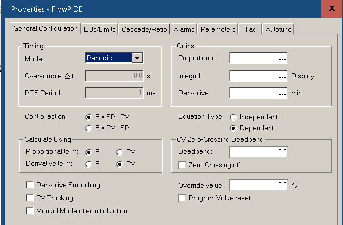
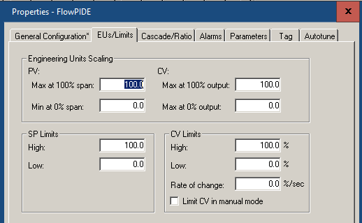
At this point, let’s click on the EU’s/Limits tab. Because we will be scaling the value externally, we’ll leave these settings at default.
Finalize your edits, and you are ready to move on to the next session to tune the PID loop!
— Ricky Bryce