
Introduction to Tuning the Simulator with an Enhanced PID (PIDE) Instruction
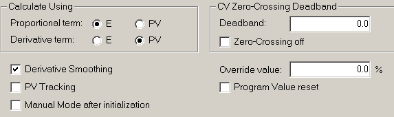
There are a few things to keep in mind when tuning the simulator with the Enhanced PID (PIDE) Instruction. First of all, the PIDE uses Function blocks. You will need to make sure you have activated the Function Block feature of Studio 5000. Secondly, the PIDE instruction bases it’s calculations by Velocity. Velocity PID’s use change in error rather than error for some calculations. For example, let’s say our error is 10%, and controller gain is 1. When we change the controller gain to 2, there is no immediate change in output. However, from now on, any change in error will change the proportional output twice as much.
In the last section, we set up the PIDE instruction using a function block. At this point, we’ll tune the PIDE.
Set up a Trend Chart
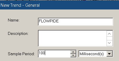
Before we begin, let’s create a trend chart that monitors FlowPIDE.SP, FlowPIDE.PV, and FlowPIDE.CV. Right click the Trends folder to start a trend. We’ll just name this as FlowPIDE, and the sample period is 100ms.
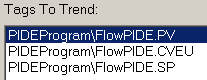
On the next screen, choose the scope (program) that your tags reside in. Add the tags to the “Tags to Trend” box.
Click Finish, then go to the chart properties. Set the X-Axis tab for a time span of 5 minutes. Likewise, go to the Y-Axis tab, and set the axis for a predefined scale. This will use the min/max settings of each pen on the pens tab. This already defaults as 0 to 100%.
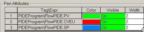
Go to Pens and set up the colors of your tags.
Click “Run”. You should see data on your trend chart, thought it won’t be doing much just yet.
Initialize the CV for Tuning the Simulator with the Enhanced PID
Since this is a velocity PID, we’ll initialize the Control Variable. That way, it starts off where we would expect it to be. Right on 0.
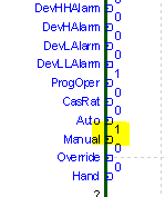
First, turn on your FlowProgProg bit. The FlowAutoReq is still 0.

This should now have the instruction in Manual Mode.
Next, go to the configuration of the instruction with the ellipsis. Turn on the CVInitReq bit, hit enter, then shut it back off, and hit enter.
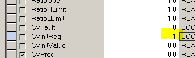
This should have initialized the PIDE instructions’ Control Variable to a value of 0.
Now, turn on your LevelProgAutoReq bit.

We should now be fully functioning in Auto Mode.
Tuning for Kc
Remember our goal is to increase the value of Kc until the loop becomes unstable. Once the loop becomes unstable, we’ll record the natural period. We’ll use the natural period for other settings later on. After we record the natural period, we will cut Kc in half.
Start your trend chart, so we can start recording data. Minimize your trend chart.
To begin, set your load to 10% on the Flow simulator.
In the properties of your PIDE instruction, we’ll set the Kc to 0.25. Let’s see what happens on the trend chart.
Perform an online edit, and change the setpoint to 50. We’ll leave the setpoint at 50 for the rest of this exercise.
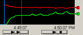
As you can see, our Control Variable increased, and everything appears to be stable. You will have some normal, small fluctuations in a flow process.
Let’s increase Kc to 0.5. After that, let’s cause a disturbance by increasing the load to 50%. Watch the graph, then reduce the load back to 10%.
As you can see, the loop is still stable.
Let’s perform the same experiment with Kc at 1. Try to change your load to 50% after changing the controller gain. If the PV Settles, change the load back to 10%.
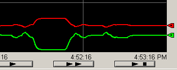
We started to see a slight overshoot from where the process variable will eventually settle. Let’s increase Kc to 1.5, and observe the results. Test your transition to 50%, then back to 10% again.
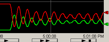
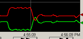
As you can see. We survived the transition to 50%, however, we became unstable during the load transition back to 10%. Let’s record the natural period. In this case, it’s around 10 seconds, which is .17 minutes. We will use this value for calculating the integral, and derivative later on. For now, it appears that our best value for Kc is around 0.75.
Notice that the peaks of the PV and CV are 180 degrees out of phase. When a loop is unstable, and the peaks are directly opposite of each other, the instability is from Proportional Gain. On the other hand if the peaks are offset by just 90 degrees, the instability is usually from your integral setting. If your integral is too high, the PV follows the CV slightly when the loop is unstable.
Finding Ti for Tuning the Simulator with Enhanced PID
Obviously, our Kc value is now stable (except for minor variations in flow). However, our process variable is far below our setpoint of 50. The integral action will make up the difference. The integral ads to the process variable every so often based on error. How often this happens will be our setting for the Ti Variable. The units for Ti are in Minutes per Repeat. Again, a repeat is based on how much error we have. As the error gets smaller, Integral still adds to the control variable. If the process variable crosses the setpoint, then the integral action is negative. It is recommended to set Ti to the natural period in minutes of the oscillations. In this case, we’ll set Ti to 0.17 and observe what happens. Remember, Kc is at 0.75 now.
Once your loop stabilizes, try a load transition to 50%. Observe your chart, then set the load back to 10% after it stabilizes. You might want to change your X axis to a span of 15 or 20 Minutes to observe the progress of our changes.
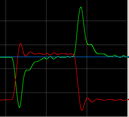
Obviously, fast load transitions cause a lot of error. However, your settings are able to correct for this error, and bring the Process Variable back to the Setpoint. If our process cannot handle this much error, then we simply need to slow down the load transitions. We could run into danger of overfilling the tank. You could prevent a disastrous event by cutting off the feed pump if the level nears 100%. Another option is to divert the excess into another tank.
If you are using Independent mode, then your variable is Ki. This is usually in repeats per minute, or repeats per second. For repeats per minute, simply use this formula. Ki=Kc/(Ti*60).
Finding Td for Tuning the Simulator with Enhanced PID (Derivative)
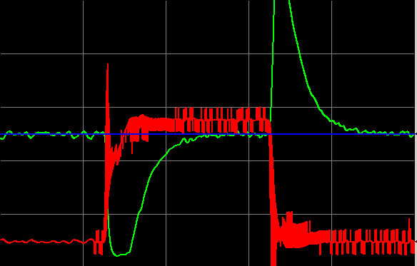
Usually, you will not use derivative in a flow control process. As you can see, the process variable is a bit noisy. This can cause excessive control action. Derivative is predictive. Derivative is based on the rate of change of the process variable (or error). Think of derivative as opposing a change in error. This applies whether the slope is positive, or negative. By setting derivative, we set up how far into the future we want to predict. Based on a given slope, a prediction over a longer time will have more effect on your control variable. As a rule of thumb, Td = 1/8th of the natural period. In other words, 1/8th of Ti. In this case, that would be about 0.02. Add derivative, and see what happens during your load transition to 50%, and then test the load transition back to 10%.
Aside from the derivative action causing the control action to be all over the place, it took us longer to get to the setpoint. This is because the derivative action opposes a change in the process variable (as per our configuration settings). Another option is for derivative action to oppose a change in error.
Obviously, we have an overactive control variable. Derivative smoothing could help with this. In the properties of your PIDE instruction, turn on Derivative Smoothing.
Perform your transitions to 50% then back to 10% again.
You will see that it does help, but we still have a lot of activity on the control variable. Normally, in a flow process, we’ll just leave the derivative at 0. Go to the properties of the PIDE instruction to turn off the derivative action.
If you are using Independent mode, then use this formula to convert Td to Kd in ControlLogix.
Kd = Kc * Td * 60
Summary
To Summarize, we simply raised Kc until the process variable was unstable in certain load transitions. That that point, we recorded the natural period. We reduced Kc to half. We set the Ti variable to the natural period in minutes. Derivative would be 1/8th of Ti if we decide to use it.
— Ricky Bryce