
Introduction to PID tuning with Ziegler-Nichols method (rule based variation)
In this section, we’ll tune a PID with the Ziegler-Nichols Method. This will be a rule based variation. Previously, we discussed a trial and error based method. Recall that we increased Kc until the loop was unstable. At this point, we record the natural period. After that, we divide Kc by 2, and Ti was our natural period of the oscillations. We are going to perform this exercise using our simulator.
A big disadvantage of PID with Ziegler-Nichols Method is that we must use open loop control. This means the PID will not have control of the control variable as we tune the loop. Additionally, the loop must be stable, and we will apply step changes. The loop must have some natural stability. For example, when the process variable is higher, the losses are higher.
As always, when tuning a loop, you must have protections in place. You very well could loose control of the output. Especially since we need to open the loop for this method.
Realize that if you re-tune a loop in a cascade configuration, you may have to tune the other loops in the configuration as well.
Remove all PID Influence from the Control Variable
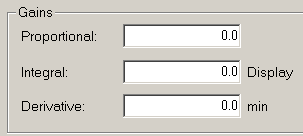
Since this this is a velocity PID, we will set Kc, Ti, and Td to zero. The output will remain constant. To emphasize, we have no control of the output at this point. It always remains constant.
Now, wait for the Process Variable to settle.
On this trend chart, green is the process variable. Similarly, red is the control variable. Blue represents the setpoint.
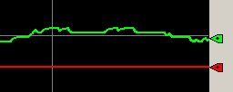
As you can see, our Control Variable is flat. It has no action.
Apply a Step Change
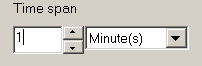
We’ll apply a small bias to the FF input of the PIDE instruction. The purpose of this step change is to cause a disturbance, so we can record some properties of our process variable. Since this method is heavily dependent on making sure our timing is accurate, change your X axis to a span of 2 minutes.
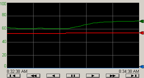
Apply a Feed Forward bias of 1%. Watch the graph. Stop the chart once your process variable stabilizes.
At this point, we need to record some data from the chart.
Recording Variables for tuning PID with the Ziegler-Nichols Method
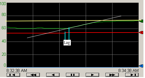
The first thing we’ll need to do is draw a tangent at the divergent point. Basically, this is the average slope of the graph.
Our Lag time is about 2 seconds.
At this point, we need the Time Constant (tau).
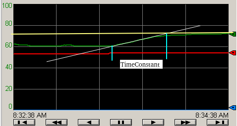
Our time constant is 30 seconds. This should be the amount of time it takes for our process variable to get to about 63% of it’s final value.
Variables for Tuning
To summarize, I’ll list the variables we have recorded so far.
- Recall that the change in output was simply 1%.
- gp is the percent change in PV, which is 12.
- Td is our lag, which is 2 seconds, or .03 Minutes.
- Tau is the time constant, which was 30 seconds., which is .5 Minutes.
Calculate the Gains
To calculate our starting gains, we simply need to plug these variables into an equation.
If want only want to use a proportional controller, out:
- Kc=Time Constant / (%PV Change * Lag)
Most of the time, we will use proportional and integral together. In that case, we would set the gains using the following formulas
- Kc= 0.9 * Time Constant / (%PV Change * Lag)
- Ti = 3.33 * Lag
If you decide to use all 3 elements of PID, then use the following formulas. The units are in minutes.
- Kc = 1.2* Time Constant / (%PV change * Lag)
- Ti = Lag * 2
- Td = Lag / 2
Now, let’s calculate our values if we are using just a PI Controller:
Kc = .01875
Ti = .111
Let’s plug in these numbers to see how the loop will respond. Using this method, our Kc is much less aggressive, and these numbers rely heavily on Integral. In other words, the Proportional gain is lower, and the integral gain is faster.
You can now remove the FF Bias. Hard code the setpoint to 50 in our flow controller, and see if the loop is stable. We also need to restart our trend chart.
Test Your Work
Try a setpoint of 20. Once the loop stabilizes, change your setpoint back to 50 to test our disturbances.
Remember that red is the control variable. Green represents our process variable. Green is the setpoint.
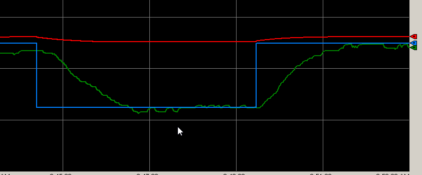
Clearly, we are able to achieve the setpoint within a reasonable amount of time.
Summary
In short, we removed the controller’s ability to provide a change in output. We did this by setting Kc, Ti, and Td all to zero. Next, we provided a step change by using Feed Forward (FF) Bias. We recorded the process lag time. At this point, we also recorded the time constant. That is the amount of time it took the PV to reach 63% of it’s final outcome. We also recorded the final resting value for the process variable. Once we had our values written down, we simply plug these values into the above equations to tune the loop.
— Ricky Bryce