
Introduction to Tuning PlantPAx P_PIDE with Simulator
Before Tuning PlantPAx P_PIDE, please reset your simulator. This way, we’ll get back to a known configuration. To reset the simulator, use your test button until you get to the reset option. Then press Up then TEST again.
In the last sections, we’ve already set up our function block logic and HMI displays. Additionally, we pointed the HMI Objects to tags in the processor, and scaled our analog values.
Configure the PID Faceplate
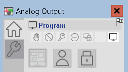
First of all, be sure your P_AOut instruction is in program control mode.
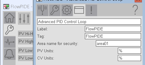
Before we begin, we need to set up a few things on the P_PIDE faceplate. First of all, let’s set up our Tag and Label. That way, we are sure which PID we are working on.
Go to Maintenance | Advanced Properties | HMI Configuration. We’ll simply name this as FlowPIDE.
Next, we’ll set up which PID Equation we wish to use. Independent mode calculates P, I, and D separately. With Dependent mode, a change in P affects the rest of the equation as well. You are probably using both types in various equipment. Independent is more traditional, but there are still a lot of independent PID loops. Basically, the equation you use depends on your preference.
For this exercise, we will use Dependent mode. Keep in mind the equation we use will affect our final values for Integral and Derivative. On the engineering tab, go to page 4. Set your mode to dependent.
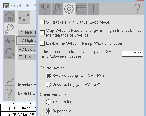
Additionally, on this page, you will set the action. Forward acting or reverse acting. This is how the PID calculates the error. For this simulation, we want reverse acting. We need more output to reduce the error. Remember, the error is not absolute. That is to say, if the process variable crosses the setpoint, the error becomes negative (in which case, the error is still getting lower).
At last, you are ready to tune the loop.
Find Kc
For this exercise, we’ll use a heuristic method. In other words, we’ll use trial and error. This is usually the fastest way to tune the loop. It’s important to realize that a heuristic method is not random. We simply find the critical value of proportional gain that causes instability. We know the loop is unstable when we have continuous oscillations.
To begin, let’s set the load on your flow simulator to 20%.
We are still in operator control mode.
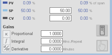
On the tuning tab, enter an operator setpoint of 50%. In the same way, set the Proportional Gain (Kc) to 1. Integral and derivative are zero. Let’s observe the result of our settings.
Switch to Auto Mode.

As you can see, nothing happens.

The reason nothing happens is because this loop is based on velocity. In other words, the change in the control variable will only happen if we have a change in error. Since there is no change in error, any value we apply to Kc at this point will not move the process variable. We need to go to manual mode, and find an output value that will raise our process variable to a point that we can tune the loop.
Switch back to Manual mode, and place a value of 25 into the CV. By slowly raising the CV, I’ve found that 25% output will bring our process variable into mid range for tuning.
Now, switch back to auto mode.
Kc=1
At this point, we need to apply a step change. This way we can observe the effects of disturbances in the system. We can do this by changing the setpoint, or the load. For this example, let’s just decrease the setpoint to 25%. Keep in mind, we are still in operator mode. This means that we can change the setpoint from the faceplate.
As you can see, we had a disturbance in our system. The process variable did finally settle on a value, and is stable.
Kc=1.5
Since we did see a few “hops” in the process variable, this means we are probably getting close to the critical value for Kc. Let’s increase Kc slightly to 1.5, and move the setpoint back to 50%.
Kc=1.75
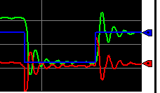
We are definitely approaching instability. Let’s try 1.75. Again, reduce your setpoint to 25.
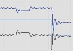
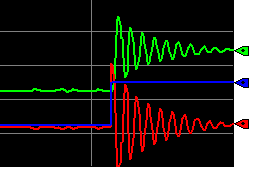
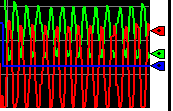
As you can see, a Kc setting of 1.75 did cause continuous instability.
At this point, we need to record the natural period, then decrease Kc by half. Meanwhile, we will record the natural period. This is the number of minutes it takes to get from peak to peak of trough to trough. Basically, this is 10 seconds. This would be 0.17 minutes.
Reduce Kc by half, to 0.88
Let’s apply your step change with a setpoint of 50.
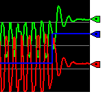
As soon as we applied our new value for Kc, we became stable very quickly. Notice we are still below the setpoint. We’ll fix that when we add integral.
Calculate Integral-Ti (Tuning PlantPAx P_PIDE with Simulator)
Most controllers simply use Proportional and Integral. In short, Kc alone does not usually hold the setpoint.
As a rule of thumb, our Ti in minutes per repeat will be equal to the natural period (which is .17). Keep in mind, this is simply a starting point. We use Ti in the dependent equation. If you use independent mode, then we need to convert Ti to Ki. Always pay attention to the units. If your Ki is in repeats per minute, then use the following formula: Ki=Kc/(Ti*60). If your controller uses repeats per minute, then simply use Kc/Ti.
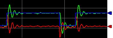
Let’s enter .17 for integral, and then apply some step changes. We’ll drop the setpoint to 25%, and the PID should recover, and your process variable should be around 25. After that, raise the setpoint back to 50%. Observe how the PID responds.
Clearly, we recovered from the disturbance. However, we do have some minor fluctuations until the Process Variable settles. Let’s see if we can fix that by reducing Kc somewhat. Let’s try Kc=0.75. Try your transitions again.
As you can see, we basically have one less hop when the setpoint was at 50. This time, leave your setpoint as is, and we’ll cause a disturbance by changing the load. We’ll make sure the loop is still stable under load transitions.
The characteristics of the load changes are different from the setpoint changes. However, we are still able to maintain the setpoint.
Calculate Derivate–Td (Tuning PlantPAx P_PIDE with Simulator)
Generally, you will not use derivative often unless you have a special purpose for it in your plant. Derivative anticipates future error. It does this based on the slope of the process variable (or error depending on your settings). Derivative opposes a change in the process variable. It works by extending the slope to find what the error will be in the future. Obviously, for any slope, the further we predict into the future, the more effect derivative will have.
For dependent mode, we simply divide Ti by 8 to get Td. If you use independent mode, then follow this equation for Td in Minutes: Kd = Kc * Td * 60 As I’ve said before, if your units are in seconds instead of minutes, then your formula would just be Kc * Td.
Since our natural period was .17 minutes, we need 1/8th of that amount for our Td. In this case, the value is .02.
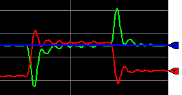
Let’s add .02 as our derivative and watch the result.
Check your load transitions to 50%, then back to 25% to cause a disturbance.
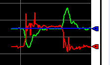
We were able to get to the setpoint, however, we have excessive controller action. This could cause excessive wear on the control equipment. In turn, this requires extra maintenance. A better way to anticipate load transitions is usually with Feed Forward (FF). We’ll discuss this in a later session. For now, let’s remove the derivative, and set the value to 0.
Summary
In short, we simply found the value of Kc that causes continuous oscillations. At this point, we record the natural period, and cut Kc in half. After that, we use the natural period in minutes as our Ti variable. Likewise, we use 1/8th of the natural period for Td if we decide to use it. If your controller has Ki and Kd variables, you are probably using independent mode. In that case follow the formulas above for conversion to those variables.
Keep in Mind that if you are in program control mode, your program will control the setpoint. Usually, you will do this by making PSet_SP visible, and feed a value into this node from your logic. Additionally, in a cascading configuration, the master PID loop would change the cascade setpoint of the instruction. In the next section, we’ll cover cascading PID in PlantPAx.
— Ricky Bryce