
Introduction to Tuning a PID for Tank Level
Tuning a PID for Tank Level has some challenges that are different than a standard PID tuning procedure. In the first place, a tank level is not self regulating. It’s an integrating process. In other words, if the system is slightly out of balance, the error will continue to become worse over time.
This is different than a self-regulating process such as temperature. With temperature control, the higher our temperature, the more losses we have. For example, we have ambient losses, electrical losses, and losses due to the load. Therefore, a given change in output will only change the temperature by a certain amount.
Consider the following process of a linear tank:
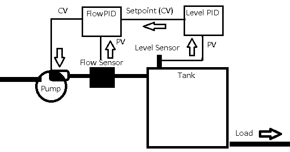
In this example, our level PID will provide a setpoint to the flow controller. This is a cascading loop. Since we already have the flow controller tuned, we will concentrate on the level PID controller.
In this example, we will take open loop control of the tank (manual) for tuning the PID. We might need to perform a step change to determine the dynamics of the process. If you don’t have the ability to perform a step change, you can calculate the dynamics by determining the volume of the tank, and the flow rate of your pump.
The tuning method we’ll use here is for slow moving processes. For surge tanks, which are fast moving processes you will need a different method.
Warning about Tuning a PID for Tank Level
Obviously, we do not want to overfill the tank. Likewise, we don’t want the tank to run empty if we are running production. It’s important to realize that varying the tank level will also vary the head pressure to the load. Before we begin, talk to the operator to see how much deviation we are allowed on the tank level. Take care not to exceed these limits when tuning.
Always have a safety in place in the event that we do overfill the tank. One option is to kill the flow pump if the tank gets close to overfilling. Keep in mind that if we run the tank empty, you might want to make sure your load has the ability to pull product from another source.
In this case, we are using a simulator and not tied to a real world process.
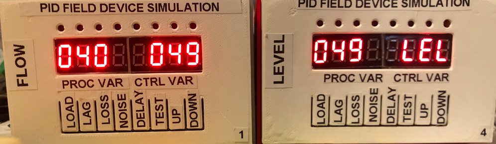
Set up the Simulator
At this time, we’ll be using the simulators that we built. We’ll start with default settings, however, set the loss on your level simulator to zero. Additionally, be sure the lag is zero, and in the test menu, set the tank size to “large”. (large=1).
Find the Dynamics of the Process
At this time, we need to find out how much a change in gain affects our change in level. This will be our process gain variable, or Kp.
Keep in mind that we need to take care not to exceed the level deviation the operator gave to us. If you can only deviate by 5%, for example, simply fill the tank by 5%, then empty it by 10% to give us the best sample for our tuning. At this time, we are not running production, though. That is not a concern.
We need to get two values from our step change. We need to know our process lag, and the process gain. The process lag is the amount of time it takes for the process variable to start moving after we change the control variable. The process gain will be the change in slope of the process variable divided by the change in output. Remember, the output is the control variable.
Remember this is an integrating process. For this reason, we must return the output to the original value as soon as possible. This will minimize our deviation.
Change Output by 5%
Generally, we’ll do our calculations for slope in %. This means you may have to scale your values into percent before performing your calculations.
As you can see, our process is balanced. When we start with a balanced process, the math is much simpler. Because our previous slope is flat (0), we simply divide the slope our change produces by the output that produced it. Keep in mind that we need the signs of our values to be correct. For example, if the slope is down, then our slope is negative.
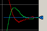
The green line is our process variable. Likewise, the blue line is the setpoint.
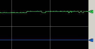
At this time, our PV is above the setpoint. Therefore, it would make sense to perform a negative step change. Well reduce the output by 5% in manual mode. Let’s do this just long enough to get a lag and slope without exceeding our process limitations.
Observe the Lag and Slope
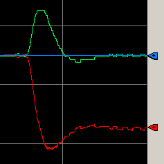
Zoom in to find the dynamics of the process. We represent the output, or Control Variable by the red line.
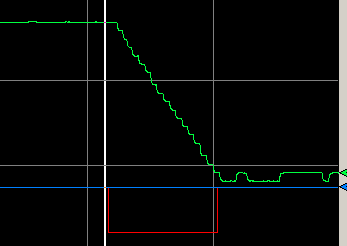
If you move your mouse over various parts of the graph, you will see the value of each pen at a certain time. In this case, I’ve placed the value bar over the exact time that we changed the CV. I found the lag time to be 6 seconds. It’s important to realize that our dependent mode equation uses minutes, so we need to convert 6 seconds to .1 minutes.
At last we need the slope. We define the slope as rise over run. The Process variable went from 67% to 60%. This took 1.1 minutes (one minute, 6 seconds.) Therefore our slope is (-7/1.1), or -6.36. Recall that our change in power was -5%. Therefore -6.36/-5 = 1.272. Kp = 1.272.
It’s important to realize you may want to try this a few times to make sure the slope is repeatable. If your process variable is very noisy, or you have a sticking valve, you might try to get an average of your slopes. Of course, a better method would be to repair any mechanical issues first before tuning.
Calculate the Tuning Variables
At this point, we have enough information to find our values. There are several variations of rule based methods, but we’ll use one that gives us some customization to our loop. That way, if the loop is unstable, or too slow, we can simply change our safety margin.
For the following formulas, we’ll use these variables:
- SM = (Safety margin) Typically, this will be 2 to 5. 2 will be faster, while 5 will be slower.
- ri = (integration rate) Change in slopes / change in output Remember we started with a stable process. Therefore, this is simply our slope.
- Td = (lag time) This is the time it takes our process variable to start changing after we change our output.
I found the following formulas at: https://blog.opticontrols.com/archives/697
To calculate tuning constants for a PI (only) controller:
Kc = 0.9 / (Safety margin * Integration Rate * Lag)
Ti = 3.33 * Safety Margin * Lag
Td = 0
If you wish to use derivative as well:
Kc = 1.2 / (Safety Margin * Integration Rate * Lag)
Ti = 2 * Safety Margin * Lag
Td (controller setting) = Lag / 2.
Test Your Work for Tuning a PID for Tank Level
Finally let’s plug our values in. We’ll just use a PI controller in this case. Therefore Kc = .94 & Ti = .4
As you can see, we quickly achieved our setpoint.
Let’s cause a disturbance, and reduce the load on our level controller to 25%.
As you can see, even though our process variable is a bit noisy, we did come back to the setpoint.
Surge Tanks
Realize that surge tanks have a faster response time, and therefore a different formula. For surge tanks, try this link, which I found at https://blog.opticontrols.com/archives/918
Summary
In short, tank levels are an integrating process, and therefore require a different tuning method. We simply performed a bump test in manual, and observed the lag, and slope. After that, we just plugged those values into formulas to find the tuning variables. Keep in mind that you must be careful with a tank controller in manual mode. The level can become too high or low very quickly. Always consult the operator to see what deviation your process can tolerate.
— Ricky Bryce