
Introduction to Independent PID with ControlLogix
In this section we’ll set up an Introduction to Independent PID with ControlLogix. Realize the equation is different than the dependent mode. For detailed information on the PID instruction, visit the ControlLogix Instruction Set Reference Manual. The PID instruction is in chapter 13.
With an Independent (traditional) PID, each componenet of P, I, and D are calculated separately.
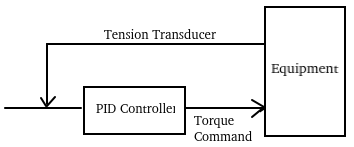
Consider the following process: We want to maintain a constant tension on our product. We will send a torque command to the equipment to maintain the tension at a specific setpoint. We’ll use our PID Simulator to emulate this process.
Finding Raw Values for Independent PID with ControlLogix
Before we begin, we need to know what our raw values are for torque and tension. There are several ways to do this.
First, we could refer to the product documentation. We would need to know what signal the transducer provides to the analog module. Also, we need to know the raw data the module provides to our controller tag for that signal. We can use the module user manual for this. Likewise, we need to know what signal range our torque controller expects. Then, we use the manual to figure what raw value we need to send to the analog output module to provide this signal.
Secondly, if we already know the voltage or current range of our field devices, we can scale the data on board the analog modules. The SLC modules do not support this. However, if you have ControlLogix modules, simply go to the properties of the modules to configure the scaling for each channel.
Thirdly, we could simply provide maximum pressure to our transducer, and see what value appears in the controller tag. Be careful experimenting with different values for output modules though. You could damage your equipment or cause harm to other employees.
Find the Raw Max
At this point, we’ll simply press the test button on our simulator to see what values we get. Press test once for 0% tension. Press test again to see 100% tension.
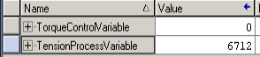
As you can see, our raw max for tension is 6712. Using the user manual, we will know the maximum value for output Torque is 32767.
Note: If your signal is 4ma to 20ma, be sure to write down both the min and max values. They will likely not be zero.
Configure the Task
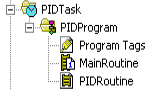
Set up a new task named “PIDTask”. Since the PID needs a stable time base, we’ll make this a periodic task, and set the period to 10ms. Likewise, set up a new program named “PIDProgram”. The PIDProgram will contain a MainRoutine, and a PIDRoutine.
Go to the properties of the PIDProgram, and be sure to configure your MainRoutine as “Main”. Your Task setup should be similar to this example:
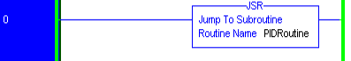
Add a JSR instruction into the MainRoutine, so the subroutine will execute.
Scaling Analog Data
This step is not required. The PID instruction itself can scale data. However, it does make the PID easier to understand if we think in terms of percent instead of raw data.
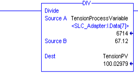
If your raw data at 0% is not zero, then your math will be a little more complex. You can use the CPT instruction to apply an offset and a multiplier. However, if zero raw data represents 0%, we can simply use MUL and DIV instructions for our scaling. Create a tag called “TensionPV”. Setup your DIV instruction in the PIDRoutine as follows:
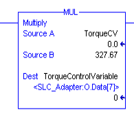
Likewise, we need to scale the torque. Create a tag called “TorquePV”. It’s important to realize we are scaling backwards this time. We are scaling from percent back to raw data. This time, we’ll use the MUL instruction.
PID Instruction
At last we’ll add the PID Instruction to the PIDRoutine. We’ll create a tag called “TensionerPID”. Configure the PID as follows:
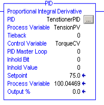
The process variable reads our tension. We are not using Tieback. This would be an output setting when in manual mode. We are not using cascading loops, so this is not a master. The inhold bit and inhold value is for bumpless restart. We are not using these values. Set them at 0. Obviously, the setpoint is our desired tension reading. The process variable, and output% simply display the values of our current tension and torque.
Configure the Independent PID with ControlLogix
Tuning Tab
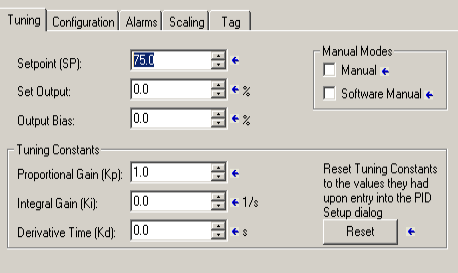
Press the Ellipsis (three dots) to get into the configuration screen of the PID instruction. Set up the “Tuning” tab as follows. We’ll start with a setpoint of 75%, and a controller gain (Kp) of 1.
Configuration Tab
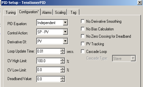
Next, go to the “Configuration Tab”. We’ll be using the Independent PID equation in this section. Our Control Action is reverse acting (SP-PV) This means that our error is positive if the process variable is below the setpoint. Remember that we set up the PIDTask to execute every 10ms. Therefore, we set our loop update time to be .01 Seconds. The high limit of your Control Variable is 100%.
Scaling Tab
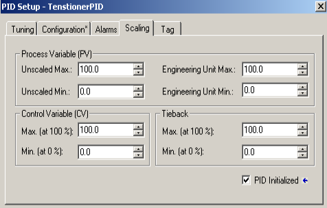
At this point, we’ll go to the “Scaling” Tab. All of our values will scale from 0 to 100%.
Trending
At this point, we need to set up a trend chart. This allows us to monitor the response of any gain changes in our PID.
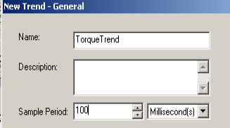
Right click the “Trends” Folder in your Controller Organizer window. Create a new trend chart. For this example, a sample period of 100ms is sufficient. If your process is very fast, you might leave your sample period at 10ms.
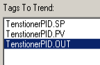
Click “Next”, and add your TensionerPID.SP, PV, and OUT as your tags to trend. Next click “Finish”.
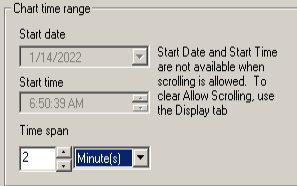
Open your trend chart, then right click the chart to go to the chart properties. Set your X Axis for a span of 2 minutes.
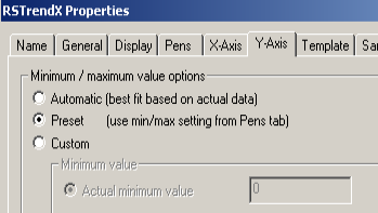
At this point, go to the Y Axis tab. Configure the Y Axis (Scaling) to use the Preset min/max settings from the PENS Tab.
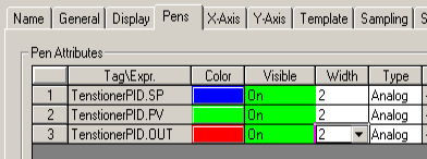
At last, go to the “Pens” Tab, and set up your preferences for each pen. For consistency with this document, the setpoint is blue. Our Process Variable is green. The Control Variable is red. Be sure the Min/Max for each pen is 0 to 100%. I’m setting the width to 2 for better visibility on the trend chart.
Tuning the Independent PID with ControlLogix
Finally, we are read to tune our loop. Recall that our controller gain is 1, and integral and derivative are at zero. We’ll use Allen Bradley’s rules of thumb for tuning this loop. Our goal is to increase Kp until the loop becomes unstable. At that point, we’ll record the natural period of the oscillations. This is the number of seconds it takes for an oscillation to complete one cycle. At this point, we’ll cut Kp in half, and use the natural period to calculate a starting point for the other tuning parameters.
Controller Gain (Kp)
Kp=1
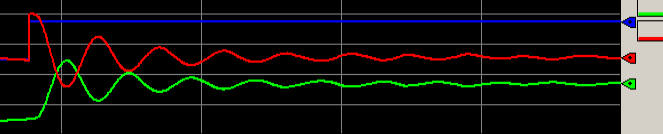
We’ll start with a controller gain (Kp) at 1. What this means is that if the error increases by 1%, then the output will also increase by 1%. Our error times the Kp will be the output. Remember our goal is to find the value of Kp that causes the loop to become unstable. Be sure to click “Run” on your trend chart.
We need to perform a step change. Bumping the process allows us to see the results of our tuning parameters. Change the setpoint to 50. When the process variable settles, change the setpoint back to 75.
As you can see, our loop does stabilize.
Kp=1.25
Let’s try the same procedure with Kp set at 1.25.
As you can see, even though the loop became more unstable, it did stabilize.
Kp=1.5
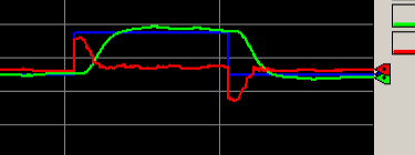
Let’s try Kp=1.5
Out loop is now basically unstable.
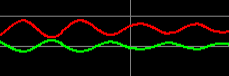
At this point, we record the natural period. This is 12 seconds. Also, we’ll cut Kp in half. Our new value for Kp is .75
Integral Gain (Ki)
You noticed above that with Kp only, we did not achieve our setpoint. In some cases, we are very far from it. However, Kp has done what it’s designed to do. It will provide an output based on error. If we did achieve the setpoint with Kp only, then there would be no error. Our output would have gone to zero. This is where integral comes in. Notice the units for our integral. This is in repeats per second. Therefore a higher value of Ki will produce a faster response time. However, if we set Ki too high, the loop becomes unstable again.
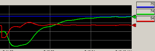
A good rule of thumb in this case is to use the following formula: Ki=Kp/natural period in seconds) This would be .75/12, or .0625. Set Ki to .0625 with Kp set at .75. Wait for the Process variable to settle. Change your setpoint. Ensure the process variable will always achieve the setpoint.
Obviously, our settings do work for a SP of 75.
Change your setpoint to 50.
We also get a great response time.
Calculate Derivative (Kd)
We don’t always use derivative. In most cases, we can get by with just Proportional, and Integral. Derivative opposes a change in the process variable (or error depending on the setting). Derivative is based on the rate of change. In other words, if the process variable drops quickly, the derivative action will immediately raise the control variable. Derivative predicts what our error will be in the future. We adjust how far into the future that our derivative will look. Obviously, the further we look into the future for a given slope, the more our difference of error will be.
If you decide to use derivative, a good rule of thumb is to use this formula for a starting point. Kd = Kp*(one eighth of natural period). In this case, our Kd is 1.125
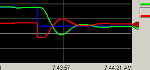
Let’s enter this number as our derivative gain. Try your load transitions again to test the result.
As you can see, we still get a good response, however our process variable does move a bit more slow. This is because derivative opposes a change in the process variable.
Summary
To summarize, with an independent mode PID, each components is calculated separately. A rule of thumb is to run Kp up until the loop becomes unstable. At this point, record the natural period of the oscillations. Cut Kp in half. Ki will start at Kp/natural period). Kd will start at Kp*(1/8th of the natural period).
For more information, visit the PID Category Page!
— Ricky Bryce