
Intruduction to Tuning a Simulator with the PID Instruction (using ControlLogix)
In the previous section, we set up the PID instruction in ladder logic. We created a Task, a Program, and a Routine. Not only did we set up the configuration, but also the scaling. At this point, we are ready to tune the PID loop. We’ll start off with default settings on the simulator.
Trending for Tuning the Simulator with a PID Instruction
Before we begin, we need to set up a trend chart. This allows us to track the process variable, control variable, and setpoint. Right-click the trends folder to create a new trend. The trend folder resides just above the I/O configuration.
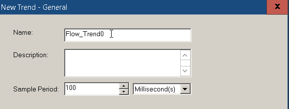
Let’s name this as “Flow Trend”. Set the sample period to 100ms. The sample period is how often the tags will refresh. Click “Next”.
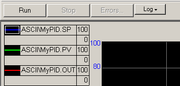
It’s important to realize that your scope will be different than what is in this documentation. Choose the program that you created your PID tag in (if this is a program scope tag). Otherwise choose the controller name if it’s a controller scoped tag. Select the Setpoint, Output, and Process Variable from “MyPID” tag. Finally, click “Finish”.
In the chart properties, go to “Pens”. In this case, I’ve set my preferred colors, and width of each pen. Also be sure to check the scaling for the Min and Max values.
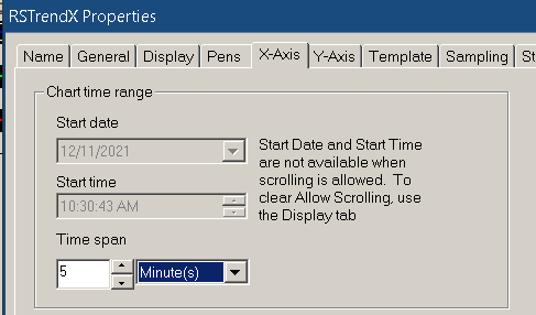
We’ll set up the X axis tab to track a 5 minute period.
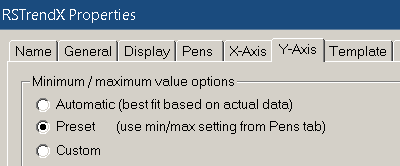
Keep in mind that we already set the scaling for each pen. At this point, go to the Y axis tab, and choose “Preset” for your scaling.
Click “Apply”, then “OK”.
Finally, click the “Run” button to start your trend.
Tuning for Proportional Gain (Kc)
At this point, we are ready to go back to your PID instruction. Click the ellipsis on the instruction, and go to the “Tuning” tab. Set Kc to 1. Ki, and Kd are zero at this time. Our goal is to find out which value of Kc will cause the loop to become unstable. Once the loop is unstable, we can gather some information to tune the other PID parameters.
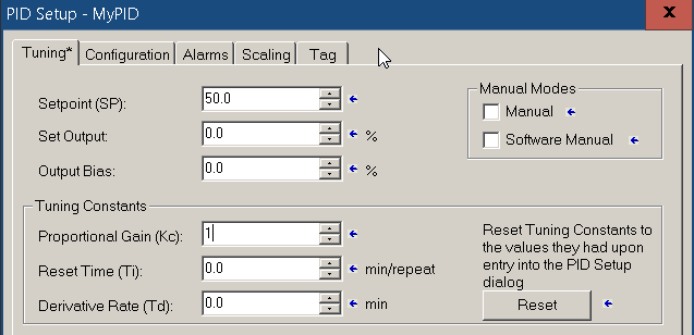
Press “Enter” then “OK”.
Go back to your trend chart, and observe the result of Kc=1.
As you can see, the loop seems to stabilize.
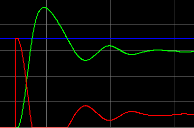
Let’s introduce a disruption. Change the load on your simulator to 60%.
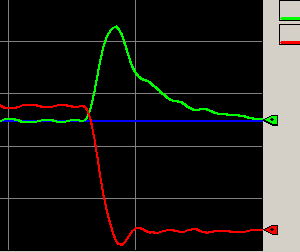
You will see that the loop is still stable. Because we need to find out which value of Kc causes instability, increase your Kc to 2.
As you can see, the value of Kc that causes instability is 2. We didn’t even need a disturbance to discover this. If it was stable, though, we might want to verify the stability with a disturbance, such as a load change. We could narrow this down, and try 1.5, but what we are looking for is a ballpark figure to start. We can fine tune the PID later on.
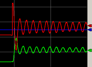
At this point, record the natural period. This will be either peak to peak or trough to trough. In this case, the natural period is 20 seconds, which is .33 Minutes.
Cut your Kc value in half. Kc will be equal to 1.
It’s important to realize that even though our loop is stable, the process variable is not even close to the set point. We will correct for this with integral.
Tuning for Integral (Ti)
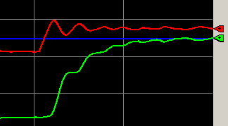
When you are using the Dependent mode, the starting integral value is very simple. Your starting integral value is the natural period. In this case, Ti = .33. However, if you are using the Independent mode, then the conversion for Ki would be Kc / (60*Ti). This would be .05. Keep in mind that Ti is the natural period. Set Ti to .33, and let’s observe the result. In any event, we should always get back to the setpoint.
As you can see, we have achieved a setpoint, and are stable.
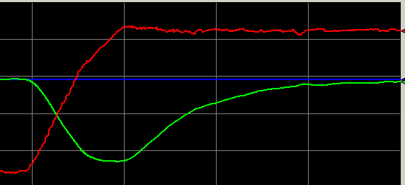
Verify the stability by reducing the load back to 5%.
When we dropped the load, our control variable spiked. This is because it takes the valve some time to respond. However, we did become stable again at our setpoint of 50%.
Tune for Integral (Kd) (Tuning the Simulator with the PID Instruction)
We don’t always need Derivative. Generally this causes more problems in a process than it solves. In some loops, however, it is necessary. Derivative basically opposes a change in the process variable. Derivative will look into the future for a predicted error, and adjust the output accordingly. The derivative setting is how far into the future we will predict the error to be for a given slope.
As a rule of thumb, in dependent mode, the derivative (Td) will be 1/8th of the natural period. In this case, that would be (.04) If you are using independent mode, we will use a formula to calculate a starting value. This is Kc * Td * 60. Kc is the controller gain, and Td is 1/8th of Ti. Keep in mind that Ti is the natural period. For this example, if we were using independent mode, the Td value would start at 2.4 (1 * .04 * 60).
Let’s add Td, and see if we notice a difference in response. We’ll need to create a disturbance to test this, so increase the load back to 80%.
Our curve is wider. This is because derivative opposes a change in the process variable. This happens both on the down slope and the up slope. As our process variable decreases, derivative adds to the output. As our process variable increases, derivative reduces the output.
Let’s take our load back to 5%.
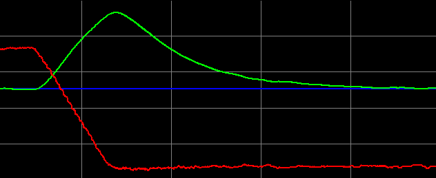
Once again, our curve is wider and smoother. It does take longer, however to get back to the setpoint.
Try to tune this loop on your own now, using various settings for lag. This will simulate different processes with different lag times, and give you more experience with tuning PID loops!
Manual Modes
There are two manual modes for the PID instruction in Ladder Logic: Manual (Hardware Manual), and Software Manual It’s important to realize that if you select both modes at the same time, the Hardware Manual mode overrides Software Manual. Generally, you can choose one of these modes from check boxes on the tuning tab.
For Hardware Manual mode, be sure your tieback scaling is correct on the scaling tab. At this point, you can change the value of the tieback tag to set the output. You can enter a tieback tag on the instruction face. Another way to enter hardware manual mode is to set the MO bit in the instruction’s tag.
Additionally, you have software manual mode. Before entering software manual mode, be sure the “Set Output” value is where you need it to be! To change the Set Output value in your program, simply write to the .SO sub element of your PID’s tag. Enter software manual mode through a checkbox on the “tuning” tab. Another way to enter software manual mode is to turn on the SWM bit in the instruction’s tag.
In the next section, we’ll cover Cascading PID.
— Ricky Bryce