
Introduction to Cascading PIDE (Enhanced)
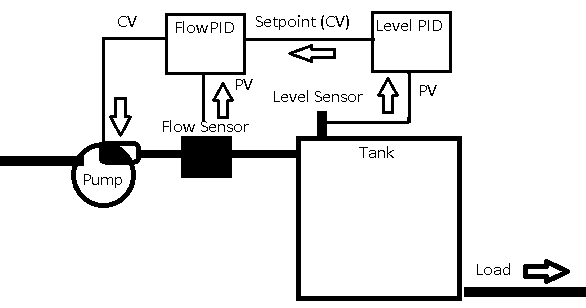
In this section we’ll discuss Cascading PIDE (Enhanced). We’ll set this up using the simulator. We’ll need two simulation units with a 1000uF capacitor across the PV of the flow simulator. Be sure to wire the PV of the flow simulator to the CV of the level simulator. Set the load on the flow simulator to 50%. Likewise, set the load on the Level controller to 0% for now.
Realize that this particular example is self regulating. In other words, as the tank level rises, it creates more pressure on the bottom of the tank. This naturally results in more outlet flow. This allows us to have a self-regulating process so we can concentrate on how cascading control works. Non-Self regulating processes require a different tuning method, which we will discuss in a different section.
Visit this link if your tank level is a true integrating process.
Because PIDE is a function block instruction, you need to make sure function blocks are activated in Studio 5000. In the last section, we set up a simple flow controller. In this section, we’ll set up cascading PIDE instructions. We’ll use a one PIDE to control flow. A second PID will adjust the flow to maintain a tank level.
Keep in mind that PIDE is a velocity controller. In short, it calculates from the change in error. On the other hand, position PID calculates by current error.
We’ll set up cascading PID to monitor a tank level, and adjust flow. Our goal is to maintain a specific level. Basically, the level controller will be changing the setpoint on the flow controller. When tuning cascading loops, we start with the lowest loop in the hierarchy first. In this case that was the flow controller. In the last section, we’ve already tuned our flow pide.
Configure Tags for Cascading PIDE (Enhanced)
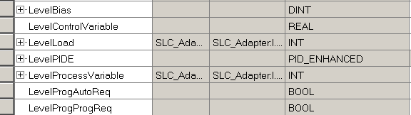
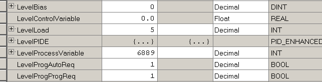
We’ll need a few tags for the PIDE instruction to work. To begin, create a tag called LevelProcessVariable. This tag will be an alias. It will point to a channel on your input module that measures a tank level.
We’ll also create a tag for the PIDE instruction to hold it’s status. We’ll just create a tag called LevelPIDE. This will have the PID_Enhanced data type. Once again, we’ll create a third tag called LevelControlVariable. We’ll give this tag the “REAL” Data Type.
As you can see, there are a few more variables to create: LevelBias as DINT, LovelProgAutoReq as BOOL, LevelProgProgReq as BOOL. Lastly, create LevelLoad that points to your FeedForward analog input. You don’t need this for the PIDE to work, but we’ll use this value later on.
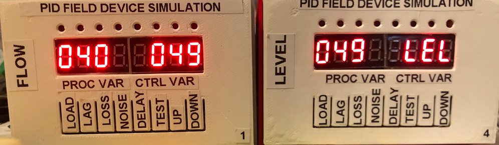
Before we continue, we need to find the raw minimum and maximum values for the LevelProcessVariable. Go to “Monitor Tags”. Now press the TEST button on your simulator. The LevelProcessVariable will reflect the low raw value. Press TEST again. At this point, you should see the high raw value. Be sure to write these down. Another way to get the low and high raw values is to consult the user manual for your module. Also, check the configuration of your analog input module.
In this case, our low value was near zero. Our high raw value is 6889. Press TEST 5 more times to exit test mode.
Add your Logic for Cascading PIDE (Enhanced)
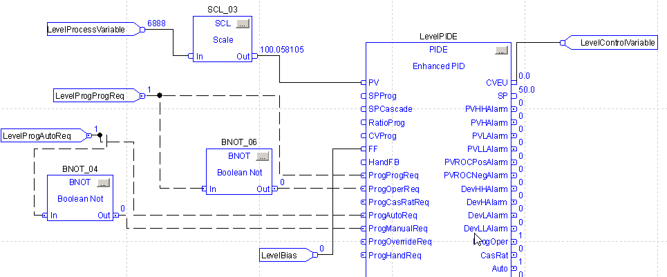
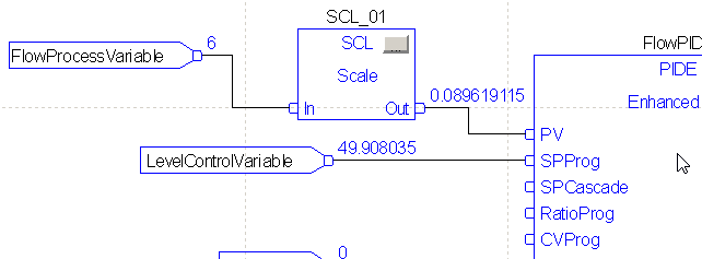
In the last section, we already set up a PIDE instruction for Flow Control. We’ll just add another sheet to our existing function block. We’ll need five IREFs, 2 BNOTs, 1 SCL, an OREF, and a PIDE instruction. Set up your sheet as follows. For now, we’ll have a setpoint of zero. Configure your SCL instruction to scale our raw data to a percentage. Recall that you wrote down your raw min and max earlier. Be sure to change your PIDE’s tag to “LevelPIDE”. If we hadn’t already created this tag, we could simply rename the tag that Studio 5000 creates.
Although the PIDE can scale the process variable directly, we’ll use the SCL to simplify our configuration inside of the PIDE.
Configure the PIDE Instruction
At this point, we need to click on the ellipsis on the PIDE Instruction.
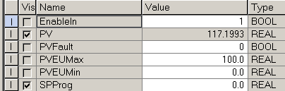
Under “General Configuration”, set up the PIDE as follows. We’ll start with a proportional gain of 1. Integral is in Minutes/Repeat, and should be 0. Likewise, the Derivative setting is zero to start. Since this loop is reverse acting, the control action will be SP-PV.
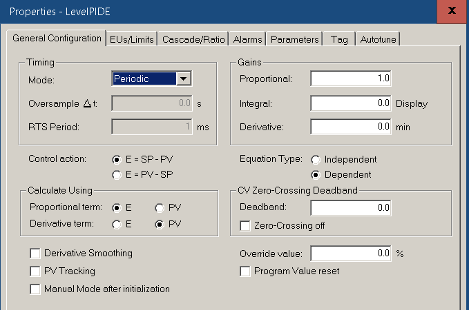
At this point, we’ll go to our EU’s and Limits. Since we are scaling data outside of the instruction, we’ll leave these all at 0 to 100%. Since cascading PID provides imperfect control, we could set limits for the CV% and it’s rate of change. For now, we’ll leave this feature at 0.
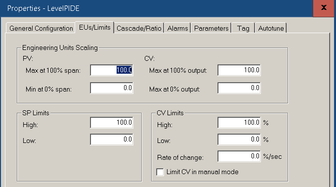
Since the units on the flow controller are the same as the units on the level controller, we do not need to configure a ratio. Press “Apply” and “OK”.
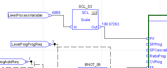
Don’t forget to feed the LevelProcessVariable into the PV Node for the FlowPIDE.
Finally, change the logic to your flow controller. The LevelControlVariable will be the setpoint into your flow controller.
Finalize your edits.
Initialize the Control Variable
Since this is a velocity loop, we should initialize the control variable. The purpose of this is to make the instruction act like a position based loop at first. That is, until we change the gains.
Set SPProg to 0 in the parameters of the instruction.
With our setpoint at zero, and our proportional gain at 1, turn on your CVInitReq bit. With a CVInitValue of 0.0, this will hold the CV at zero, which is our set point for the flow controller Therefore, our tank should eventually empty. Wait for the tank to empty. We will know it’s empty when the LevelProcessVariable is near 0
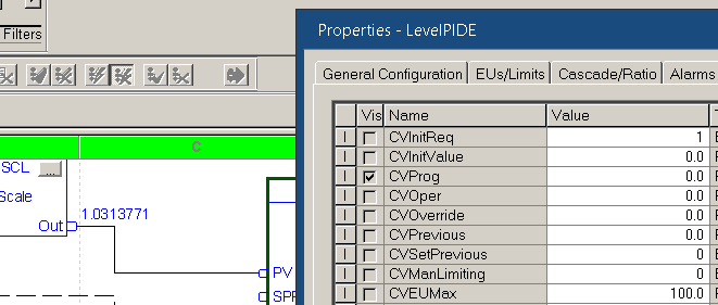
Shut your CVInitReq bit back off. Be sure to hit enter, then apply. The CV should now be initialized, free of any previous influences.
Set up a Trend
As before, we’ll set up a new trend chart. This will help with tuning the loop.
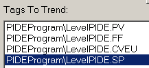
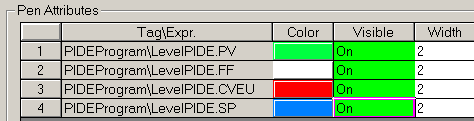
Under “Tags to Trend”, add these three tags: LevelPIDE.PV, LevelPIDE.FF, LevelPIDE.CVEU, and LevelPIDE.SP.
Set the X axis to a period of 10 minutes. The Y axis will use the “Preset” min and max from the “Pens” tag. This already defaults from 0 to 100%.
On the Pens tab, configure the colors for each pen.
Be sure to click “Run” to start your trend chart.
Tuning the PIDE
At last, we are ready to tune our loop. Our goal is to achieve the setpoint of a tank level. We will have some random process fluxuations, but we’ll tune the loop to stay within 5% of our target level.
Warning: We’ll make a few assumptions when tuning this loop. First of all, we have protection in the event the tank overfills. Secondly, if our tank is empty, the load will pull product from another source. If this is not the case, then you must take care not to allow the tank to become completely full or empty. You would have to use the rule based method, or apply changes in a way to keep the processvariable near the setpoint. In our case, this is simply a startup, and we are free to tune for the worst case scenario. We have freedom to tune this particular loop without adverse reactions in the process.
Finding Kc (Proportional Gain)
Keep in mind that this is a cascading loop, and will be a little bit more difficult to tune. Also, cascading control is not always perfect. Combine that with the fact that this loop is velocity based, and we’ll have to do a few experiments and changes in load to find the correct values.
Set your load on the flow controller to 50%, and we’ll start off with a small load on the level controller at 5%.
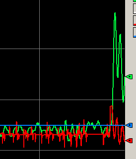
Recall that we started off with a proportional gain of 1. Let’s see what effect this will have if we raise the the SPProg parameter to 50.
As you can see, our loop is very unstable. Not only that, but our CV is saturating at zero. The saturation will cause a problem with our tuning. Set Kc to .5.
Move our SPProg back to 0, then re-initialize the loop. After the process variable settles, stop the initialization. Once again, move your SPProg to 50. be sure to hit enter then apply after making the change. Check your trend chart.
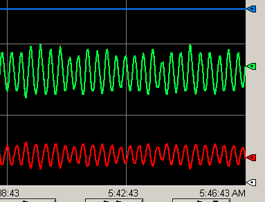
Since we are still unstable, and not saturating, simply move Kc to .25. Once again check your trend chart.
As you can see, aside from mild flow fluctuations, we have now become stable. The point is clearly defined from the point that we switched Kc from .5 to .25. The natural period of the oscillations is about 20 seconds, or .3 Minutes.
Note: If Kc causes your gain to be so low that the process variable does not increase, you can apply some Feed Forward (FF) Bias. This will cause your PV to increase into a range where you can easily tune the loop. This is a challenge we could encounter when tuning velocity PID loops.
Calculate Integral (Ti) for Cascading PIDE (Enhanced)
Recall that our natural period was .3 minutes. As a rule of thumb, a good starting point for Ti is the natural period of the oscillations. Remember, we are using the dependent PID equation. To calculate integral for independent mode, use the following formula: Ti = Kc/(Ti*60). (For repeats per second).
Let’s try our Ti setting of .3.
Change the load on your LEVEL simulator to 40%.
As you can see, we get back to the setpoint. However, we do have a small amount of random noise on the process variable.
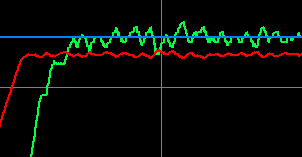
At this point, we have tuned the loop, and achieved our goal of maintaining the tank level within 5%.
Calculate Derivative (Td)
As I’ve said before, we don’t always use Td. In many cases, it is detrimental. However, if we want to add derivative for the dependent equation, it will be 1/8th of the Ti. This is a good starting point. Let’s set derivative to .0375, and see what the effect is.
Since our process variable has some noise, we have an overactive controller. This can cause wear and harm to our pump, and other components. This could simply be due to the low resolution of our process variable.
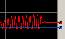
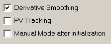
Let’s try Derivative smoothing. This is an option in the configuration of your PIDE instruction.
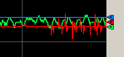
Right away, you see a change in the reaction. The on the left half of the image below, derivative smoothing is shut off. The right half shows our action with derivative smoothing.
As you can see, in this case, our problem is now much worse. We do not want to use derivative in this process because of the natural changes in our process variable.
For, this loop, we’ll set derivative back to 0.
If you are using an independent controller, you would convert the Td to Kd (in seconds).
Kd = Kc * Td * 60, where Td is 1/8th of the natural period.
Summary
To summarize, we found the value of Kc that started causing oscillations. Once we had oscillations, we documented the natural period of the loop. If we don’t have a high enough PV to tune the gain, we could add some Feed Forward (FF) Bias to allow us to tune the loop. Next, we used the natural period in minutes as our Ti variable. We also decided that we don’t want to use derivative in this case.
In the next section, we’ll discuss Feed Forward, and how we can use that to anticipate changes in the system.
— Ricky Bryce